library(elicitr)
#> Registered S3 method overwritten by 'lme4':
#>   method           from
#>   na.action.merMod car
Many of the concepts introduced in
vignette("continuous_variables") are also applicable to
categorical variables, and the name of the functions are the same but
have the prefix cat instead of cont. However,
there are some differences in the workflow for loading and analysing
data collected during the elicitation of categorical variables. This
vignette will guide you through the process of loading and analysing
categorical data.
Datasets
There are three datasets included in the package for demonstration
purposes: ?topic_1, ?topic_2, and
?topic_3:
topic_1
#> # A tibble: 120 × 5
#>    name            option   category   confidence estimate
#>    <chr>           <chr>    <chr>           <dbl>    <dbl>
#>  1 Derek Maclellan option_1 category_1         15     0.08
#>  2 Derek Maclellan option_1 category_2         15     0
#>  3 Derek Maclellan option_1 category_3         15     0.85
#>  4 Derek Maclellan option_1 category_4         15     0.02
#>  5 Derek Maclellan option_1 category_5         15     0.05
#>  6 Derek Maclellan option_2 category_1         35     0.02
#>  7 Derek Maclellan option_2 category_2         35     0.11
#>  8 Derek Maclellan option_2 category_3         35     0.18
#>  9 Derek Maclellan option_2 category_4         35     0.02
#> 10 Derek Maclellan option_2 category_5         35     0.67
#> # ℹ 110 more rows
topic_2
#> # A tibble: 100 × 5
#>    name              option   category   confidence estimate
#>    <chr>             <chr>    <chr>           <dbl>    <dbl>
#>  1 Christopher Felix option_1 category_1        100     0.09
#>  2 Christopher Felix option_1 category_2        100     0.21
#>  3 Christopher Felix option_1 category_3        100     0.11
#>  4 Christopher Felix option_1 category_4        100     0.59
#>  5 Christopher Felix option_1 category_5        100     0
#>  6 Christopher Felix option_2 category_1         20     0.09
#>  7 Christopher Felix option_2 category_2         20     0.05
#>  8 Christopher Felix option_2 category_3         20     0.33
#>  9 Christopher Felix option_2 category_4         20     0.24
#> 10 Christopher Felix option_2 category_5         20     0.29
#> # ℹ 90 more rows
topic_3
#> # A tibble: 90 × 5
#>    name            option   category   confidence estimate
#>    <chr>           <chr>    <chr>           <dbl>    <dbl>
#>  1 Derek Maclellan option_1 category_1         80     0.02
#>  2 Derek Maclellan option_1 category_2         80     0.02
#>  3 Derek Maclellan option_1 category_3         80     0.01
#>  4 Derek Maclellan option_1 category_4         80     0.87
#>  5 Derek Maclellan option_1 category_5         80     0.08
#>  6 Derek Maclellan option_2 category_1         50     0.11
#>  7 Derek Maclellan option_2 category_2         50     0.09
#>  8 Derek Maclellan option_2 category_3         50     0.17
#>  9 Derek Maclellan option_2 category_4         50     0.09
#> 10 Derek Maclellan option_2 category_5         50     0.54
#> # ℹ 80 more rows
In each dataset the first column contains the name of the expert, the second the options considered and the third the categories of the categorical variable. The fourth column contains the expert’s confidence, and the fifth the expert’s estimate. Expert estimates for each option should represent probabilities or percentages, and should thus sum up to 1 or 100. Both are accepted and data scaled to 1 will be automatically rescaled to 100.
Load data
We start by creating the ?elic_cat object with the
function cat_start(). As for the continuous variables, this
objects stores the metadata of the elicitation process:
my_categories <- c("category_1", "category_2", "category_3",
                   "category_4", "category_5")
my_options <- c("option_1", "option_2", "option_3", "option_4")
my_topics <- c("topic_1", "topic_2", "topic_3")
my_elicitation <- cat_start(categories = my_categories,
                            options = my_options,
                            experts = 6,
                            topics = my_topics)
#> ✔ <elic_cat> object for "Elicitation" correctly initialised
my_elicitation
#>
#> ── Elicitation ──
#>
#> • Categories: "category_1", "category_2", "category_3", "category_4", and
#> "category_5"
#> • Options: "option_1", "option_2", "option_3", and "option_4"
#> • Number of experts: 6
#> • Topics: "topic_1", "topic_2", and "topic_3"
#> • Data available for 0 topics
This elicitation process is for a categorical variables with 5 categories estimated for four options and three topics by six experts.
As we did for continuous variables, we can load the data with the
function cat_load():
my_elicitation <- cat_add_data(my_elicitation,
                               data_source = topic_1,
                               topic = "topic_1") |>
  cat_add_data(data_source = topic_2, topic = "topic_2") |>
  cat_add_data(data_source = topic_3, topic = "topic_3")
#> ℹ Estimates sum to 1. Rescaling to 100.
#> ✔ Data added to Topic "topic_1" from "data.frame"
#>
#> ℹ Estimates sum to 1. Rescaling to 100.
#> ✔ Data added to Topic "topic_2" from "data.frame"
#>
#> ℹ Estimates sum to 1. Rescaling to 100.
#> ✔ Data added to Topic "topic_3" from "data.frame"
As mentioned before, estimates can also sum up to 100.
topic_1_percent <- dplyr::mutate(topic_1,
                                 estimate = estimate * 100)

my_elicitation <- cat_add_data(my_elicitation,
                               data_source = topic_1_percent,
                               topic = "topic_1")
#> ✔ Data added to Topic "topic_1" from "data.frame"
Expert anonymisation is automatic but optional. If expert names are
not to be anonymised, the argument anonymise can be set to
FALSE in the cat_add_data() function.
my_elicitation <- cat_add_data(my_elicitation,
                               data_source = topic_1,
                               topic = "topic_1",
                               anonymise = FALSE)
#> ℹ Estimates sum to 1. Rescaling to 100.
#> ✔ Data added to Topic "topic_1" from "data.frame"
Again, metadata are used to validate the data. If the data is not consistent with the metadata, an error message will be displayed. For example, if we try to load data with a category not defined in the metadata:
malformed_data <- topic_1
malformed_data[1, 2] <- "category_6"
cat_add_data(my_elicitation,
             data_source = malformed_data,
             topic = "topic_1")
#> Error in `cat_add_data()`:
#> ! The column with the name of the options contains unexpected values:
#> ✖ The value "category_6" is not valid.
#> ℹ Check the metadata in the <elic_cat> object.
Get data
Data can be retrieved from the elic_cat object with the
cat_get_data() function:
cat_get_data(my_elicitation, topic = "topic_1")
#> # A tibble: 120 × 5
#>    id              option   category   confidence estimate
#>    <chr>           <chr>    <chr>           <dbl>    <dbl>
#>  1 Derek Maclellan option_1 category_1         15        8
#>  2 Derek Maclellan option_1 category_2         15        0
#>  3 Derek Maclellan option_1 category_3         15       85
#>  4 Derek Maclellan option_1 category_4         15        2
#>  5 Derek Maclellan option_1 category_5         15        5
#>  6 Derek Maclellan option_2 category_1         35        2
#>  7 Derek Maclellan option_2 category_2         35       11
#>  8 Derek Maclellan option_2 category_3         35       18
#>  9 Derek Maclellan option_2 category_4         35        2
#> 10 Derek Maclellan option_2 category_5         35       67
#> # ℹ 110 more rows
Notice that the name of the expert is not anonymised in this case and
assigned to the column id.
Data can also be retrieved only for given options:
cat_get_data(my_elicitation, topic = "topic_2", option = "option_1")
#> # A tibble: 25 × 5
#>    id      option   category   confidence estimate
#>    <chr>   <chr>    <chr>           <dbl>    <dbl>
#>  1 e51202e option_1 category_1        100        9
#>  2 e51202e option_1 category_2        100       21
#>  3 e51202e option_1 category_3        100       11
#>  4 e51202e option_1 category_4        100       59
#>  5 e51202e option_1 category_5        100        0
#>  6 e78cbf4 option_1 category_1         75       31
#>  7 e78cbf4 option_1 category_2         75       27
#>  8 e78cbf4 option_1 category_3         75        9
#>  9 e78cbf4 option_1 category_4         75       17
#> 10 e78cbf4 option_1 category_5         75       16
#> # ℹ 15 more rows
Here, the data is anonymised, following what was specified when loading the data.
Data analysis
Contrary to continuous variables, there is not yet a function for plotting the raw data. However, we can plot the distribution of the sampled data.
Sample data
Data can be sampled using the function cat_sample() (see
the variable documentation for the explanation of the sampling methods).
Here we sample 100 values for each option:
samp <- cat_sample_data(my_elicitation,
                        method = "unweighted",
                        topic = "topic_1",
                        n_votes = 100)
#> ✔ Data sampled successfully using "unweighted" method.
samp
#> # A tibble: 2,400 × 7
#>    id              option category_1 category_2 category_3 category_4 category_5
#>    <chr>           <chr>       <dbl>      <dbl>      <dbl>      <dbl>      <dbl>
#>  1 Derek Maclellan optio…     0.0476          0      0.864   0.0171       0.0712
#>  2 Derek Maclellan optio…     0.0567          0      0.904   0.00235      0.0374
#>  3 Derek Maclellan optio…     0.0661          0      0.869   0.0268       0.0377
#>  4 Derek Maclellan optio…     0.0648          0      0.882   0.00612      0.0467
#>  5 Derek Maclellan optio…     0.0376          0      0.929   0.0101       0.0236
#>  6 Derek Maclellan optio…     0.0925          0      0.851   0.0102       0.0463
#>  7 Derek Maclellan optio…     0.0717          0      0.877   0.0144       0.0370
#>  8 Derek Maclellan optio…     0.0779          0      0.875   0.0125       0.0348
#>  9 Derek Maclellan optio…     0.118           0      0.769   0.0674       0.0457
#> 10 Derek Maclellan optio…     0.0904          0      0.844   0.000713     0.0650
#> # ℹ 2,390 more rows
Sampled data can be summarised for any option:
summary(samp, option = "option_1")
#> # A tibble: 5 × 7
#>   Category        Min      Q1  Median   Mean     Q3   Max
#>   <chr>         <dbl>   <dbl>   <dbl>  <dbl>  <dbl> <dbl>
#> 1 category_1 0.0109   0.0832  0.122   0.126  0.166  0.269
#> 2 category_2 0        0.00208 0.00969 0.0551 0.0915 0.338
#> 3 category_3 0.0411   0.136   0.238   0.359  0.585  0.929
#> 4 category_4 0.000152 0.00925 0.111   0.153  0.291  0.428
#> 5 category_5 0.0123   0.0579  0.308   0.307  0.474  0.748
And plotted as violin plot:
plot(samp)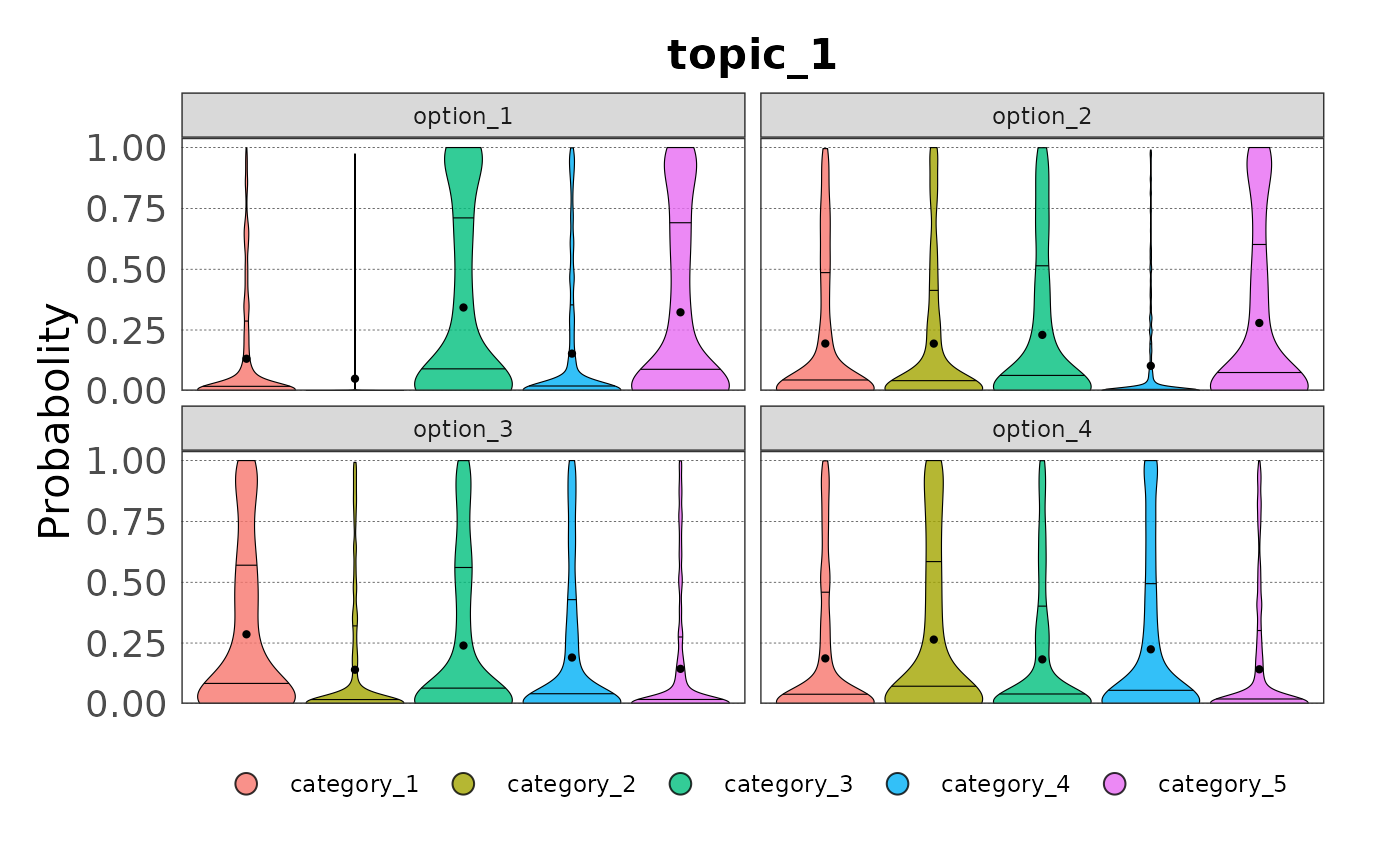
Or as beeswarm plot, which can be adapted as needed:
plot(samp, type = "beeswarm")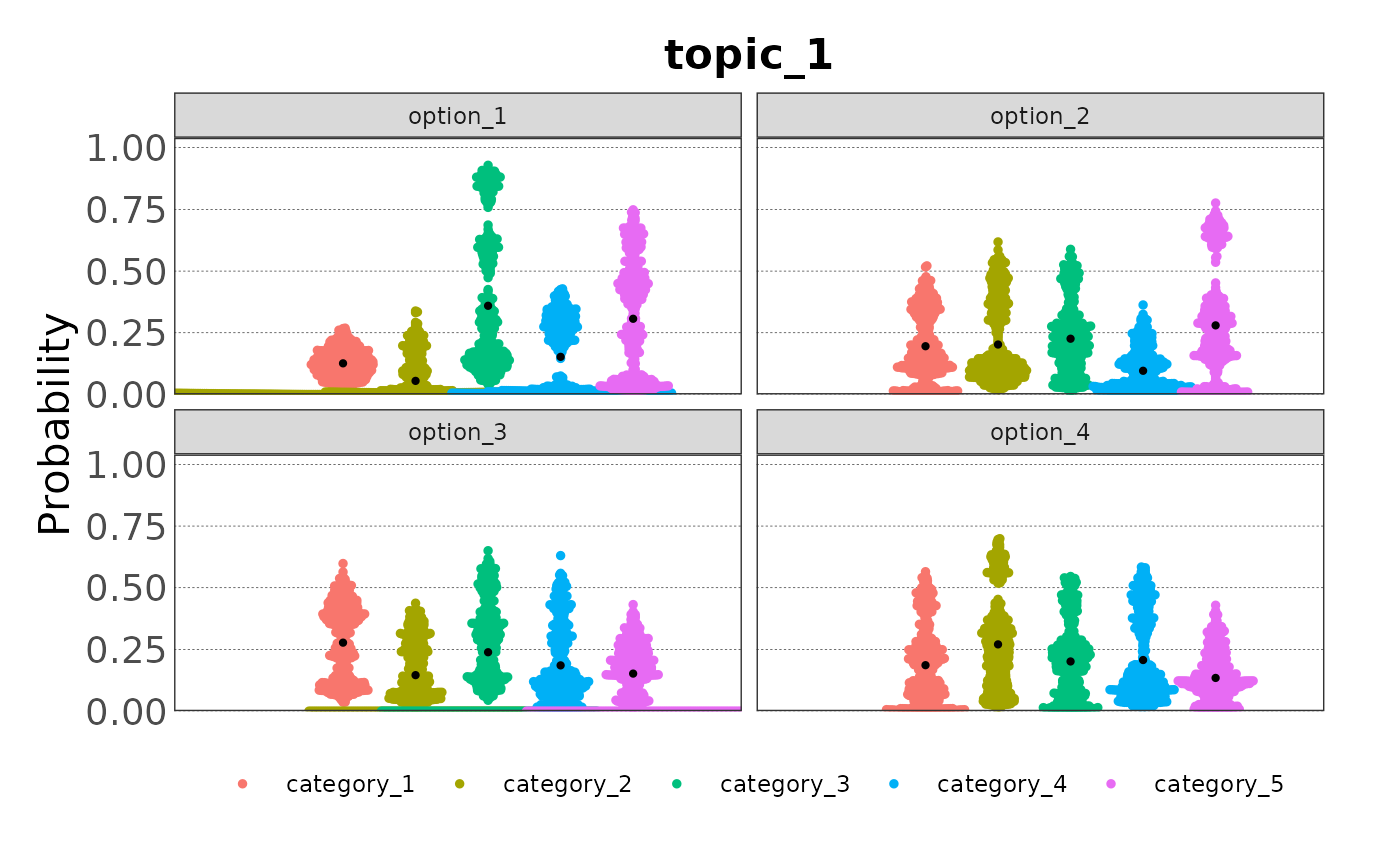
plot(samp, type = "beeswarm",
     beeswarm_cex = 0.9, beeswarm_corral = "wrap")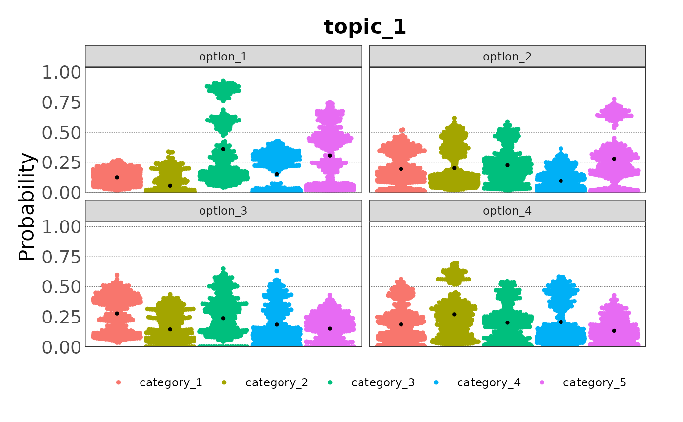
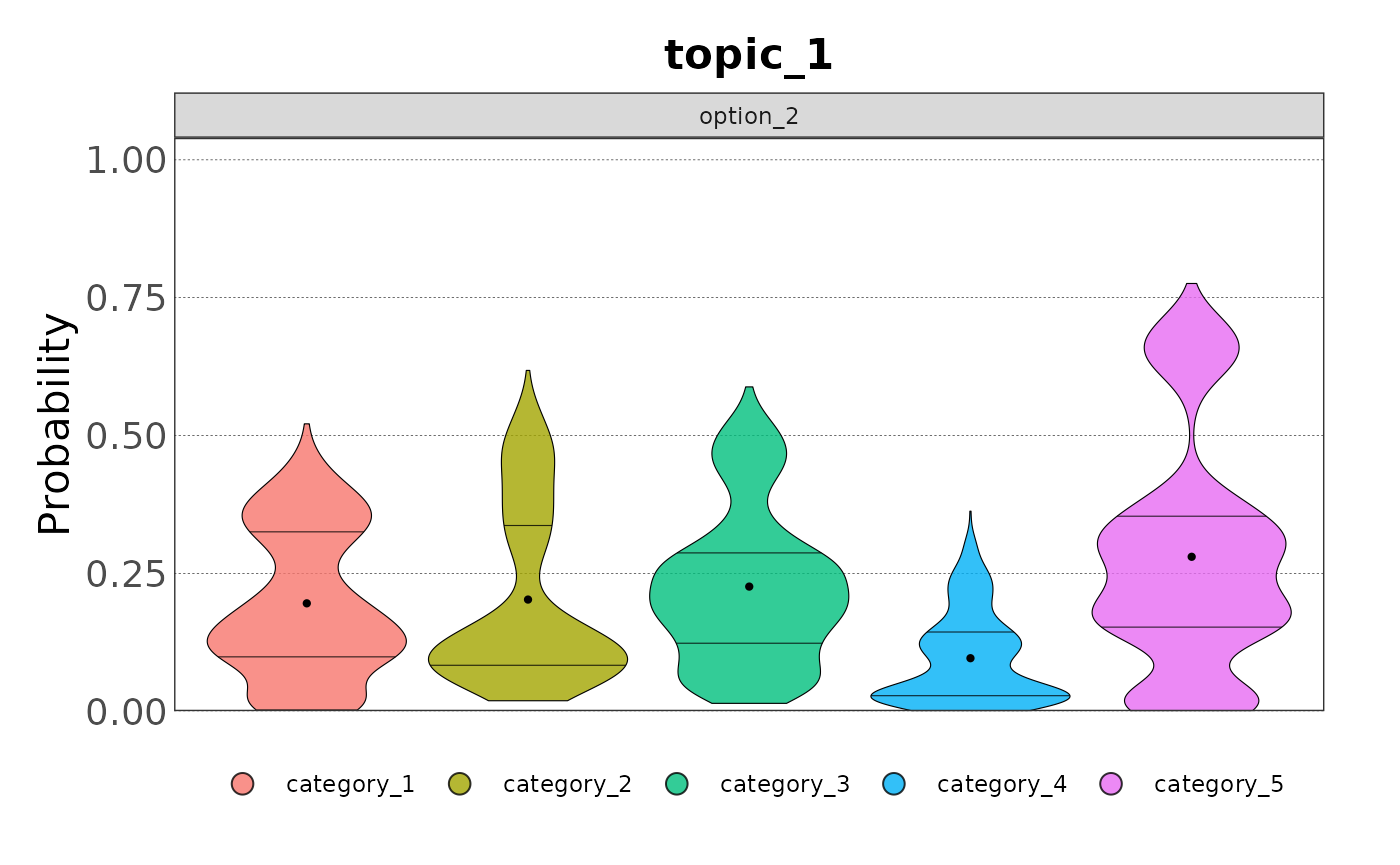
We can also plot the distribution for a specific option:
plot(samp, option = "option_2")